Dancing with the Elephants and Flying With The Bees – Apache Hive Performance Tuning

Tuning Hive and other Apache components that run in the background to support processing of HiveQL is particularly important as the scale of your workload and database volume increases. When your applications query data sets that constitute a large-scale enterprise data warehouse (EDW), tuning the environment and optimizing Hive queries are often part of an ongoing effort of your team.

Increasingly, most enterprises require that Hive queries run against the data warehouse
with low-latency analytical processing, which is often referred to as LLAP by Hortonworks. LLAP of real-time data can be further enhanced by integrating the EDW with the Druid business intelligence engine.

Hive2 Architecture and Internals.

Before we begin, I am assuming you are running Hive on Tez execution engine. Hive LLAP with Apache Tez utilizes newer technology available in Hive 2.x to be
an increasingly needed alternative to other execution engines like MapReduce
and earlier implementations of Hive on Tez. Tez runs in conjunction with Hive
LLAP to form a newer execution engine architecture that can support faster
queries.

The architecture og Hive2 is shown below:

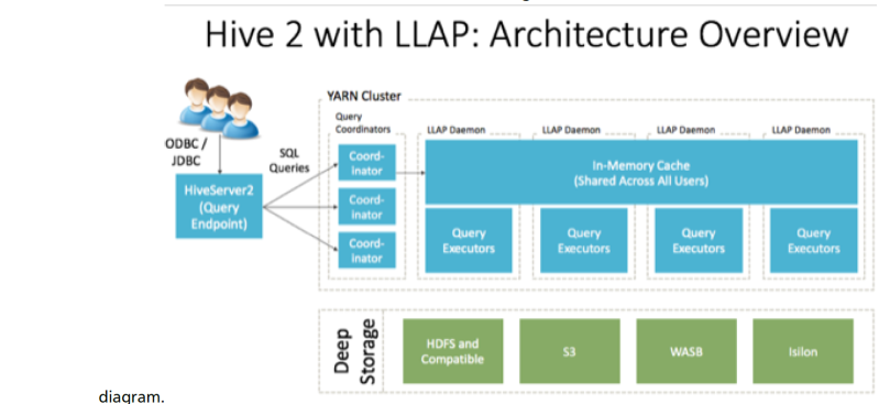
• HiveServer2: provides JDBC and ODBC interface, and query compilation
• Query coordinators: coordinate the execution of a single query LLAP daemon: persistent server, typically one per node. This is the main differentiating component of thearchitecture, which enables faster query runtimes than earlier execution engines.
• Query executors: threads running inside the LLAP daemon
• In-memory cache: cache inside the LLAP daemon that is shared across all users

Tuning Hive cluster memory

After spending some time hearing from customers about slow running Hive queries or worst yet heap issues precluding successful query execution and doing some research I learned about some important tuning parameters that may be useful for folks supporting Hive workloads.  Some of these I will get into below.

To maximize performance of your Apache Hive query workloads, you need to optimize cluster configurations, queries, and underlying Hive table
design. This includes the following:

• Configure CDH clusters for the maximum allowed heap memory size, load-balance concurrent connections across your CDH Hive
  components, and allocate adequate memory to support HiveServer2 and Hive metastore operations.
• Review your Hive query workloads to make sure queries are not overly complex, that they do not access large numbers of Hive table partitions,
  or that they force the system to materialize all columns of accessed Hive tables when only a subset is necessary.
• Review the underlying Hive table design, which is crucial to maximizing the throughput of Hive query workloads. Do not create thousands of
  table partitions that might cause queries containing JOINs to overtax HiveServer2 and the Hive metastore. Limit column width, and keep the
  number of columns under 1,000.

Memory Recommendations. 

HiveServer2 and the Hive metastore require sufficient memory to run correctly. The default heap size of 256 MB for each component is
inadequate for production workloads. Consider the following guidelines for sizing the heap for each component, based on your cluster size.

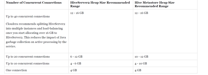
Important: These numbers are general guidance only, and can be affected by factors such as number of columns, partitions, complex joins, and
client activity. Based on your anticipated deployment, refine through testing to arrive at the best values for your environment.
In addition, the Beeline CLI should use a heap size of at least 2 GB.
Set the PermGen space for Java garbage collection to 512 MB for all.

Configuring Heap Size and GC

You can use Cloudera Manager to configure Heap Size and GC for HiveServer2

• • To set heap size, go to Home > Hive > Configuration > HiveServer2 > Resource Management. Set Java Heap Size of HiveServer2 in Bytes to the desired value, and click Save Changes.
  • To set garbage collection, go to Home > Hive > Configuration > HiveServer2 > Advanced. Set the PermGen space for Java garbage collection to 512M , the type of garbage collector used ( ConcMarkSweepGC or ParNewGC ), and enable
    or disable the garbage collection overhead limit in Java Configuration Options for HiveServer2. The following example sets the PermGen space to 512M , uses the new Parallel Collector, and disables the garbage collection overhead limit:
    -XX:MaxPermSize=512M -XX:+UseParNewGC -XX:-UseGCOverheadLimit
  • Once you made any changes to Heap and GC you will need to restart. From the Actions drop-down menu, select Restart to restart the HiveServer2 service

Similarly you can set up Heap Size and GC for Hive Metastore with the similar parameters using Cloudera Manager by going tp Home > Hive > Configuration > Hive Metastore > Resource Management.

If you are not using Cloudera Manager or on the HDInsight you can configure the heap size for HiveServer2 and Hive metastore in command line by setting the -Xmx parameter in the HADOOP_OPTS variable to the desired maximum heap size in /etc/hive/hive-env.sh .

The following example shows a configuration with HiveServer2 using 12 GB heap,  Hive Metastore using 12 GB heap,  Hive clients use 2 GB heap:


if [ "$SERVICE" = "cli" ]; then
if [ -z "$DEBUG" ]; then
export HADOOP_OPTS="$HADOOP_OPTS -XX:NewRatio=12 -Xmx12288m -Xms12288m
-XX:MaxHeapFreeRatio=40 -XX:MinHeapFreeRatio=15 -XX:+UseParNewGC -XX:-
UseGCOverheadLimit"
else
export HADOOP_OPTS="$HADOOP_OPTS -XX:NewRatio=12 -Xmx12288m -Xms12288m
-XX:MaxHeapFreeRatio=40 -XX:MinHeapFreeRatio=15 -XX:-UseGCOverheadLimit"
fi
fi
export HADOOP_HEAPSIZE=2048

You can use either the Concurrent Collector or the new Parallel Collector for garbage collection by passing -XX:+useConcMarkSweepGC or –XX:+useParNewGC in the HADOOP_OPTS lines above. To enable the garbage collection overhead limit, remove the -XX:-UseGCOverheadLimit setting or change it to -XX:+UseGCOverheadLimit .

For more on latest docs on tuning memory and troubleshootng heap\GC exceptions in Hive see Cloudera docs https://docs.cloudera.com/documentation/enterprise/latest/topics/admin_hive_tuning.html or for HDInsight see this great MS docs with configurations – https://docs.microsoft.com/en-us/azure/hdinsight/interactive-query/hive-llap-sizing-guide

Cloud VM Tracing with STrace in Azure Linux VM

strace is a powerful command line tool for debugging and trouble shooting programs in Unix-like operating systems such as Linux. It captures and records all system calls made by a process and the signals received by the process. As a person that is a huge fan of procmon tool on Windows – https://docs.microsoft.com/en-us/sysinternals/downloads/procmon  , I am pretty excited about strace on Linux. 

As such this utility can be very useful troubleshooting apps running on Azure Linux VMs as well.  Below I will show you an example of using strace for troubleshooting on Azure Linux VM.

The first thing we will do is to roll out Ubuntu Linux VM in Azure.  You can follow official Microsoft doc here – https://docs.microsoft.com/en-us/azure/virtual-machines/linux/quick-create-portal  or follow parts of my previous nmon on Azure VM tutorial here – https://gennadny.wordpress.com/2015/03/22/using-nmnon-to-monitor-linux-system-performance-on-azure/ .  Afer you done you should have an Azure Unbuntu Linux VM you can SSH into, like mine below:

If you have Windows client , use Putty to SSH into this VM.  Once you connect via SSH lets install utility:

 sudo apt-get install strace

In my case strace is installed already, so I get following output:

Next lets list all of the pids on the machine running:

sudo ps aux

Result is this:

If I wanted to take a look and find PID of particular process, axample mysql, I would run something like:

 ps aux | grep mysqld

pidof command finds the process ids (PIDs) of the named programs. It prints those PIDs on screen. Continuing on example with mysql process:

 sudo pidof mysqld

As stated this prints PID of that process:

Now we can start strace with the process ID:

sudo strace -Ff -tt -p 22695 2>&1 | tee strace-mysql.log

Now that strace is attached we can see lots of output scrolling by:

Now you can perform whatever action you need to reproduce your issue. After that, you can shut down strace with Ctrl-C.  Now you can look at what were the calls via nano editor:

sudo nano strace-mysql.log

So, as you can see we can install strace on Azure VM, attach it to offending process, repro the issue and collect log for analysis. Happy troubleshooting.

For more on strace see – https://strace.io/, https://www.tecmint.com/strace-commands-for-troubleshooting-and-debugging-linux/, https://www.thegeekstuff.com/2011/11/strace-examples  and https://linoxide.com/linux-command/linux-strace-command-examples/

 

 

Collecting Trash Revisited – Garbage Collection Essentials in .NET

In my recent past as Field Engineer working with customers I had to deal with many managed applications that had performance and stability issues due to memory usage. With .NET 4 there were definitely big interesting additions introduced to memory management , but talking to customers I believe they may have drowned out in a see of tech announcements and many developers in the field simply do not remember these. Therefore here is some basic information on Garbage Collection flavors in .NET and some ways to troubleshoot GC issues for existing applications.

Workstation vs. Server GC 

There are actually two different modes of garbage collection, which you can control using gcServer tag in the runtime configuration part of your config file. Workstation Garbage Collection is set by default. The gcServer configuration flag was introduced long ago , with .NET 2.0, and you can use it to control whether Workstation or Server GC is used on multi processor machines. With server GC, a thread for every core is created just for doing GC. There is also a small object heap and a large object heap created for each GC thread. All of the program’s allocations are spread among these heaps (more on large object heaps later). When no GC is happening, these threads are blocked and do nothing. When a GC is triggered, all of the user threads get paused, and all the GC threads wake up at highest priority and do collection in parallel. All of these optimizations lead to server GC usually being much faster than workstation GC.

So Server GC:

• Multiprocessor (MP) Scalable, Parallel
• One GC thread per CPU
• Program paused during marking

Workstation GC

• Great for UI driven apps as minimizes pausing during full GC collection
• Runs slower

Concurrent vs. Background

Now besides Server vs Workstation, there are Concurrent and Background operation modes. Both of them allow a second generation to be collected by a dedicated thread without pausing all user threads. Generation 0 and 1 require pausing all user threads, but they are always the fastest. This of course increases the level of responsiveness an application can deliver.

Concurrent Mode.

Default mode for Workstation GC and will provide a dedicated thread performing GC, even on multiprocessor machines. You can turn it off using gcConcurrent tag. This mode offers much shorter user threads pauses as the most time consuming Gen2 collection is done concurrently, on the cost of limited allocation capabilities during concurrent GC. While Gen2 collection takes place, other threads can only allocate up to the limit of current ephemeral segment, as it’s impossible to allocate new memory segment. If your process runs out of place in current segment, all threads will have to be paused anyway and wait for concurrent collection to finish. This is because Gen0 and Gen1 collections cannot be performed while concurrent GC is still in progress. Concurrent GC also has a slightly higher memory requirements.

Background Mode

Starting with .NET 4.5 this is actually default mode that replaces Concurrent.  It’s also available for both Workstation and Server modes, while Concurrent was only available for Workstation. The big improvement being that Background mode can actually perform Gen0 and Gen1 collections while simultaneously performing Gen2 collection. 

Workstation garbage collection can be:

• Concurrent
• Background
• Non-concurrent

while options for Server garbage collection are as follows:

• Background
• Non-concurrent

For more see – https://blogs.msdn.microsoft.com/tess/2009/05/29/background-garbage-collection-in-clr-4-0/, https://blogs.msdn.microsoft.com/dotnet/2012/07/20/the-net-framework-4-5-includes-new-garbage-collector-enhancements-for-client-and-server-apps/

So how do I collect my GC pause information to make decision on what mode is best for me? 

The first thing to do is take a look at the properties of the process using the excellent Process Explorer tool from Sysinternals (imagine Task Manager on steroids). It will give you a summary like the one below, the number of Gen 0/1/2 Collections and % Time in GC are the most interesting values to look at.

The other way to get very deep insight is grab an ETW trace as explained by Maoni Stephens here – https://blogs.msdn.microsoft.com/maoni/2014/12/22/gc-etw-events-1/, this is a method of looking into GC stats that I use utilizing pretty popular PerfView tool that works on top of Event Tracing for Windows (ETW). Another good tutorial on the same can be found here – http://www.philosophicalgeek.com/2012/07/16/how-to-debug-gc-issues-using-perfview/

Hope this little note is useful.

 

Forecast Cloudy – Profiling Azure Cloud Service

We can get an in-depth analysis of the computational aspects of how azure application runs by using the Visual Studio Profiler.  Below I will show you how to use Sampling performance gathering method in Visual Studio Profiler to profile Cloud Service in Azure. If you need basic information on Visual Studio Profiler start here –

https://docs.microsoft.com/en-us/visualstudio/profiling/beginners-guide-to-performance-profiling .
Sampling is a statistical profiling method that shows you the functions that are doing most of the user mode work in the application. Sampling is a good place to start to look for areas to speed up your application.

At specified intervals, the Sampling method collects information about the functions that are executing in your application. After you finish a profiling run, the Summary view of the profiling data shows the most active function call tree, called the Hot Path, where most of the work in the application was performed. The view also lists the functions that were performing the most individual work, and provides a timeline graph you can use to focus on specific segments of the sampling session.

Sampling is the most common method to application profiling, there are other methods as well, but they may come with more performance overhead or require more application instrumentation.
Make sure you enable appropriate settings when publishing your application to Azure

• In Solution Explorer, open the shortcut menu for your Azure project, and then choose Publish.
• In the Advanced Settings tab, select the Enable profiling

• Choose the Settings And select Sampling  and Enable Tier Interaction Profiling, and click OK.
• Click Next and Publish the application

Once you ran your profile you can now view profile reports. To get them do following

• Using Visual Studio Server Explorer, expand Azure -> Cloud Services ->Your_Cloud_Role ->Production (Profiling), right click on the instance, click on View Profiling Report.
• 

• It may take couple minutes for the profiling report to show up. Click on the Save icon to save a local copy for analysis

• Once you are done with profiling you may republish application without that option checked.

Happy performance hunting. For more see – http://msdn.microsoft.com/library/azure/hh369930.aspx.

Purgamentum Init Venari – Analyzing Java GC Using IBM Pattern Modeling Tool

Recently again looking at some GC issues on IBM Websphere platform for a buddy of mine I got to learn new tool – Pattern Modeling and Analysis Tool for IBM Java Garbage Collector (PMAT). This is second post-mortem IBM analysis tool I had priviledge to work with from IBM , as I previously profiled JCA – Javacore Dump Analysis Tool here https://gennadny.wordpress.com/2016/03/28/javacore-dump-analysis-using-jca-ibm-thread-and-monitor-dump-analyzer-for-java/ .

The PMAT tool parses verbose GC trace, analyzes Java heap usage, and recommends key configurations based on pattern modeling of Java heap usage.

Why do we need it?
When the JVM (Java virtual machine) cannot allocate an object from the current heap because of lack of space, a memory allocation fault occurs, and the Garbage Collector is invoked. The first task of the Garbage Collector is to collect all the garbage that is in the heap. This process starts when any thread calls the Garbage Collector either indirectly as a result of allocation failure or directly by a specific call to System.gc(). The first step is to get all the locks needed by the garbage collection process. This step ensures that other threads are not suspended while they are holding critical locks. All other threads are then suspended. Garbage collection can then begin. It occurs in three phases: Mark, Sweep, and Compaction (optional).

Sometimes you run into issues, most common are either performance issues in applications due to especially long running , aka “violent” GCs or rooted objects on the heap not getting cleaned up and application crashing with dreaded OutOfMemory error and causing you have to analyze Garbage Collection with Verbose GC on.

Verbose GC is a command-line option that one can supply to the JVM at start-up time. The format is: -verbose:gc or -verbosegc. This option switches on a substantial trace of every garbage collection cycle. The format for the generated information is not designed and therefore varies among various platforms and releases.
This trace should allow one to see the gross heap usage in every garbage collection cycle. For example, one could monitor the output to see the changes in the free heap space and the total heap space. This information can be used to determine whether garbage collections are taking too long to run; whether too many garbage collections are occurring; and whether the JVM crashed during garbage collection.

How does it work?
PMAT analyzes verbose GC traces by parsing the traces and building pattern models. PMAT recommends key configurations by executing a diagnosis engine and pattern modeling algorithm. If there are any errors related with Java heap exhaustion or fragmentation in the verbose GC trace, PMAT can diagnose the root cause of failures. PMAT provides rich chart features that graphically display Java heap usage.
The following features are included:

1. GC analysis
2. GC table view
3. Allocation failure summary
4. GC usage summary
5. GC duration summary
6. GC graph view
7. GC pattern analysis
8. Zoom in/out/selection/center of chart view
9. Option of changing chart color.

Where do I get it?

You can download this tool from – ftp://public.dhe.ibm.com/software/websphere/appserv/support/tools/pmat/ga456.jar

Running the tool
Run gaNNN.jar with the Java Run-time Environment. (NNN is the version number).
You will see following initial screen

Select and open verbosegc log

Process Log and View Summary\Reports

More detailed information on the tool can be found in presentation here – http://www-01.ibm.com/support/docview.wss?uid=swg27007240&aid=1

Jinwoo Hwang was technical leader at IBM WebSphere Application Server Technical Support that created this tool, as well as JCA. I recommend that everyone reads his articles on JVM internals – http://websphere.sys-con.com/node/1229281, http://www-01.ibm.com/support/docview.wss?uid=swg27011855 , http://www-01.ibm.com/support/docview.wss?uid=swg27018423

Hope this short note helps

Capre Noctem – Using SQL Server Diagnostics (Preview) to analyze SQL Server minidump

Microsoft just released the SQL Server Diagnostics (Preview) extension within SQL Server Management Studio and Developer APIs to empower SQL Server customers to achieve more through a variety of offerings to self-resolve SQL Server issues.

So what can it do:

• • Analyze SQL Server dump.

Customers should be able to debug and self-resolve memory dump issues from their SQL Server instances and receive recommended Knowledge Base (KB) article(s) from Microsoft, which may be applicable for the fix.

• Review recommendations to keep SQL Server instances up to date.

 

Customers will be able to keep their SQL Server instances up-to-date by easily reviewing the recommendations for their SQL Server instances. Customers can filter by product version or by feature area (e.g. Always On, Backup/Restore, Column Store, etc.) and view the latest Cumulative Updates (CU) and the underlying hotfixes addressed in the CU.

• Developers who want to discover and learn about Microsoft APIs can view developer portal and then use APIs in their custom applications. Developers can log and discuss issues and even submit their applications to the application gallery.

 

So I installed this extension and decided to give it a go with one of the SQL Server minidumps I have.

It actually correctly identified an issue and issues suggestions. So, while this may not work on every dump, it should worth trying before you start up WinDbg.

Give it a try. Hope this helps.

Let Me Count The Ways – Various methods of generating stack dump for JVM in production

As I profiled previously thread dumps in Java are essential in diagnosing production issues with high CPU, locking, threading deadlocks, etc. There are great online thread dump analysis tools such as http://fastthread.io/ that can analyze and spot problems. But to those tools you need provide proper thread dumps as input. I already blogged about many tools to do so in the past like jstack, JvisualVM and Java Mission Control. Here I will try to summarize all of the ways to capture usable thread dumps in production Java application:

• JStack

JStack remains one of the most common ways to capture thread dumps. It’s a command ike utility bundled in JDK. The Jstack tool is shipped in JDK_HOME\bin folder. Here is the command that you need to issue to capture thread dump:

jstack -l   > 

Where

pid: is the Process Id of the application, whose thread dump should be captured

file-path: is the file path where thread dump will be written in to.

Example here:

jstack -l 37321 > /opt/tmp/threadDump.txt

As per the example thread dump of the process would be generated in /opt/tmp/threadDump.txt file.

• Kill –3

 

In many customers only JREs are installed in production machines. Since jstack and other tools are only part of JDK, you wouldn’t be able to use jstack. In such circumstances, ‘kill -3’ option can be used.

kill -3 

Where:

pid: is the Process Id of the application, whose thread dump should be captured

Example:</P?

 Kill -3 37321

When ‘kill -3’ option is used thread dump is sent to standard error stream. Fpr example in apps running under Tomcat it will be <TOMCAT_HOME>/logs/catalina.out file. VisualVM Java VisualVM is a graphical user interface tool that provides detailed information about the applications while they are running on a specified Java Virtual Machine (JVM). It’s located in JDK_HOME\bin\jvisualvm.exe. It’s part of Sun\Oracle JDK distribution since JDK 6 update 7.s Launch the jvisualvm. On the left panel, you will notice all the java applications that are running on your machine. You need to select your application from the list (see the red color highlight in the below diagram). This tool also has the capability to capture thread dumps from the java processes that are running in remote host as well. In order to generate thread dump, go to Threads Tab and click on Thread Dump button.

•   Java Mission Control

 

Java Mission Control (JMC) is a tool that collects and analyze data from Java applications running locally or deployed in production environments. This tool has been packaged into JDK since Oracle JDK 7 Update 40. This tool also provides an option to take thread dumps from the JVM. JMC tool is present in JDK_HOME\bin\jmc.exe Once you launch the tool, you will see all the Java processes that are running on your local hostAs you use Flight Recorder feature on one of these processes , in the “Thread Dump” field, you can select the interval in which you want to capture thread dump.

• ThreadMXBean

 

Introduced in JDK 1.5, ThreadMXBean is a management interface for thread system in JVM and allows you to create thread dump in few lines of code in application like below:

Example

public void  dumpThreadDump() {



        ThreadMXBean threadMxBean = ManagementFactory.getThreadMXBean();



        for (ThreadInfo ti : threadMxBean.dumpAllThreads(true, true)) {



            System.out.print(ti.toString());

 

• JCMD

The jcmd tool was introduced with Oracle’s Java 7. It’s useful in troubleshooting issues with JVM applications. It has various capabilities such as identifying java process Ids, acquiring heap dumps, acquiring thread dumps, acquiring garbage collection statistics, ….

Using the below JCMD command you can generate thread dump:

jcmd  Thread.print > 

where

pid: is the Process Id of the application, whose thread dump should be captured

file-path: is the file path where thread dump will be written in to.

Example

jcmd 37321 Thread.print > /opt/tmp/threadDump.txt

For more see – https://docs.oracle.com/javase/7/docs/technotes/tools/windows/jcmd.html, https://blogs.oracle.com/jmxetc/entry/threadmxbean_a_singleton_mxbean_for , http://www.javamex.com/tutorials/profiling/profiling_java5_threads_howto.shtml , http://blog.takipi.com/oracle-java-mission-control-the-ultimate-guide/ , https://www.prosysopc.com/blog/using-java-mission-control-for-performance-monitoring/

Taking Care of the Garbage – Generational is default GC policy on newer WebSphere AS

Imagine you have a legacy Java application running in IBM WebSphere that you have upgraded finally to newer version. Yet, customer is reporting serious performance regression. Why would that be? Well, one reason maybe a change in default JVM behavior between WebSphere versions, something that one of my customers discovered the “hard way”

Garbage collection (GC) is an integral part of the Java Virtual Machine (JVM) as it collects unused Java heap memory so that the application can continue allocating new objects. The effectiveness and performance of the GC play an important role in application performance and determinism. The IBM JVM provided with IBM WebSphere Application Server provides four different GC policy algorithms:

• -Xgcpolicy:optthruput
• -Xgcpolicy:optavgpause
• -Xgcpolicy:gencon
• -Xgcpolicy:balanced

Each of these algorithms provides different performance and deterministic qualities. In addition, the default policy in WebSphere Application Server V8 has changed from -Xgcpolicy:optthruput to the  policy -Xgcpolicy:gencon.   So lets dive in a bit what this really means.

The garbage collector

Different applications naturally have different memory usage patterns. A computationally intensive number crunching workload will not use the Java heap in the same way as a highly transactional customer-facing interface. To optimally handle these different sorts of workloads, different garbage collection strategies are required. The IBM JVM supports several garbage collection policies to enable you to choose the strategy that best fits your application

The parallel mark-sweep-compact collector: optthruput, formerly default

The simplest possible garbage collection technique is to continue allocating until free memory has been exhausted, then stop the application and process the entire heap. While this results in a very efficient garbage collector, it means that the user program must be able to tolerate the pauses introduced by the collector. Workloads that are only concerned about overall throughput might benefit from this strategy.

The optthruput policy (-Xgcpolicy:optthruput) implements this strategy. This collector uses a parallel mark-sweep algorithm. In a nutshell, this means that the collector first walks through the set of reachable objects, marking them as live data. A second pass then sweeps away the unmarked objects, leaving behind free memory than can be used for new allocations. The majority of this work can be done in parallel, so the collector uses additional threads (up to the number of CPUs by default) to get the job done faster, reducing the time the application remains paused.

The problem with a mark-sweep algorithm is that it can lead to fragmentation . There might be lots of free memory, but if it is in small slices interspersed with live objects then no individual piece might be large enough to satisfy a particular allocation.

The solution to this is compaction. In theory, the compactor slides all the live objects together to one end of the heap, leaving a single contiguous block of free space. This is an expensive operation because every live object might be moved, and every pointer to a moved object must be updated to the new location. As a result, compaction is generally only done when it appears to be necessary. Compaction can also be done in parallel, but it results in a less efficient packing of the live objects — instead of a single block of free space, several smaller ones might be created.

The concurrent collector: optavgpause

For applications that are willing to trade some overall throughput for shorter pauses, a different policy is available. The optavgpause policy (-Xgcpolicy:optavgpause) attempts to do as much GC work as possible before stopping the application, leading to shorter pauses . The same mark-sweep-compact collector is used, but much of the mark and sweep phases can be done as the application runs. Based on the program’s allocation rate, the system attempts to predict when the next garbage collection will be required. When this threshold approaches, a concurrent GC begins. As application threads allocate objects, they will occasionally be asked to do a small amount of GC work before their allocation is fulfilled. The more allocations a thread does, the more it will be asked to help out. Meanwhile, one or more background GC threads will use idle cycles to get additional work done. Once all the concurrent work is done, or if free memory is exhausted ahead of schedule, the application is halted and the collection is completed. This pause is generally short, unless a compaction is required. Because compaction requires moving and updating live objects, it cannot be done concurrently.

 

The generational collection: gencon

has long been observed that the majority of objects created are only used for a short period of time. This is the result of both programming techniques and the type of application. Many common Java idioms create helper objects that are quickly discarded; for example StringBuffer/StringBuilder objects, or Iterator objects. These are allocated to accomplish a specific task, and are rarely needed afterwards. On a larger scale, applications that are transactional in nature also tend to create groups of objects that are used and discarded together. Once a reply to a database query has been returned, then the reply, the intermediate state, and the query itself are no longer needed.

This observation lead to the development of generational garbage collectors. The idea is to divide the heap up into different areas, and collect these areas at different rates. New objects are allocated out of one such area, called the nursery (or newspace). Since most objects in this area will become garbage quickly, collecting it offers the best chance to recover memory. Once an object has survived for a while, it is moved into a different area, called tenure (or oldspace). These objects are less likely to become garbage, so the collector examines them much less frequently. For the right sort of workload the result is collections that are faster and more efficient since less memory is examined, and a higher percentage of examined objects are reclaimed. Faster collections mean shorter pauses, and thus better application responsiveness.
IBM’s gencon policy (-Xgcpolicy:gencon) offers a generational GC (“gen-“) on top of the concurrent one described above (“-con”). The tenure space is collected as described above, while the nursery space uses a copying collector. This algorithm works by further subdividing the nursery area into allocate and survivor spaces . New objects are placed in allocate space until its free space has been exhausted. The application is then halted, and any live objects in allocate are copied into survivor. The two spaces then swap roles; that is, survivor becomes allocate, and the application is resumed. If an object has survived for a number of these copies, it is moved into the tenure area instead.

 

The region-based collector: balanced

A new garbage collection policy has been added in WebSphere Application Server V8. This policy, called balanced (-Xgcpolicy:balanced), expands on the notion of having different areas of the heap. It divides the heap into a large number of regions, which can be dealt with individually. Frankly I haven’t seen it used by any customer I worked with yet.

 

For more on WebSphere IBM JVM GC see – http://www.perfdaddy.com/2015/10/ibm-jvm-tuning-gencon-gc-policy.html, http://www.ibmsystemsmag.com/ibmi/administrator/websphere/Tuning-Garbage-Collection-With-IBM-Technology-for/, http://javaeesupportpatterns.blogspot.com/2012/03/ibm-jvm-tuning-gencon-gc-policy.html

Hope this helps

Javacore Dump Analysis using JCA – IBM Thread and Monitor Dump Analyzer for Java

In my previous blog posts I spent some time in illustrating tools for thread analysis for Oracle\Sun HotSpot JVM. However recently I actually had to analyze stack\javacore dumps from IBM WebSphere for hang condition and therefore had to research equivalent tools to analyze dumps from that JVM.

As we all know, during the run time of a Java process, some Java Virtual Machines (JVMs) may not respond predictably and oftentimes seem to hang up for a long time or until JVM shutdown occurs. It is not easy to determine the root cause of these sorts of problems.

By triggering a javacore when a Java process does not respond, it is possible to collect diagnostic information related to the JVM and a Java application captured at a particular point during execution. For example, the information can be about the operating system, the application environment, threads, native stack, locks, and memory. The exact contents are dependent on the platform on which the application is running.

On non IBM platforms, and in most cases, javacore is known as “javadump.” Check out my previous post of how to analyze dumps on Oracle Sun JVM via jstack utility. The code that creates javacore is part of the JVM. One can control it by using environment variables and run-time switches. By default, a javacore occurs when the JVM terminates unexpectedly. A javacore can also be triggered by sending specific signals to the JVM. Although javacore or javadump is present in Sun JVMs, much of the content of the javacore is added by IBM and, therefore, is present only in IBM JVMs.

This technology analyzes each thread information and provides diagnostic information, such as current thread information, the signal that caused the javacore, Java heap information (maximum Java heap size, initial Java heap size, garbage collector counter, allocation failure counter, free Java heap size, and allocated Java heap size), number of runnable threads, total number of threads, number of monitors locked, and deadlock information.

You can download tool from here – https://www.ibm.com/developerworks/community/groups/service/html/communityview?communityUuid=2245aa39-fa5c-4475-b891-14c205f7333c.

Once the tool is downloaded, you can run jca.jar with the Java Run-time Environment

This will open up the tool

Let’s now use File-Open and open a javacore\dump file

The tool will show a screen with a progress bar while it loads the javacore. Clicking on the javacore you just loaded in the Thread Dump List

As you can see you get huge amount of JVM settings details, as well as If the tool detected a deadlock then it will be displayed in the lower section of the Thread Dump List

and

 

Selecting the Compare Monitors option from Analysis Menu will show deadlocked threads

Another useful screen is Thread Status Screen. Here you can see RUNNABLE vs. PARKED vs. BLOCKED threads and associated stacks. This screen can be very useful in resolving slow response and hang conditions

A complete explanation of all thread states for Java 7 can be found here – https://www.ibm.com/support/knowledgecenter/SSYKE2_7.0.0/com.ibm.java.aix.71.doc/diag/tools/javadump_tags_threads.html. Once you locate the RUNNABLE threads that are executing your application code, find out which method is being executed by following the stack trace. You may get  assistance from development team if needed. Also note the Thread ID.

The following Thread in the example below is in BLOCK state which typically means it is waiting to acquire a lock on an Object monitor. You will need to search in the earlier section and determine which Thread is holding the lock so you can pinpoint the root cause.

3XMTHREADINFO      "[STUCK] ExecuteThread: '162' for queue: 'weblogic.kernel.Default (self-tuning)'" J9VMThread:0x000000013ACF0800, j9thread_t:0x000000013AC88B20, java/lang/Thread:0x070000001F945798, state:B, prio=1

3XMTHREADINFO1            (native thread ID:0x1AD0F3, native priority:0x1, native policy:UNKNOWN)

3XMTHREADINFO3           Java callstack:

4XESTACKTRACE                at org/springframework/jms/connection/SingleConnectionFactory.createConnection(SingleConnectionFactory.java:207(Compiled Code))

4XESTACKTRACE                at org/springframework/jms/connection/SingleConnectionFactory.createQueueConnection(SingleConnectionFactory.java:222(Compiled Code))

4XESTACKTRACE                at org/springframework/jms/core/JmsTemplate102.createConnection(JmsTemplate102.java:169(Compiled Code))

4XESTACKTRACE                at org/springframework/jms/core/JmsTemplate.execute(JmsTemplate.java:418(Compiled Code))

4XESTACKTRACE                at org/springframework/jms/core/JmsTemplate.send(JmsTemplate.java:475(Compiled Code))

4XESTACKTRACE                at org/springframework/jms/core/JmsTemplate.send(JmsTemplate.java:467(Compiled Code))

…………………………………………………………………………………………………………

 

Hope this helps. For more see – https://www.ibm.com/developerworks/community/groups/service/html/communityview?communityUuid=2245aa39-fa5c-4475-b891-14c205f7333c, https://www.ibm.com/developerworks/community/blogs/e8206aad-10e2-4c49-b00c-fee572815374/entry/Java_Core_Debugging_using_IBM_Thread_and_Monitor_Dump_Analyzer_for_Java?lang=en

Resolving Java Threading Issues with ThreadLogic Tool

The ThreadLogic utility is a free tool you can download to assist in analyzing thread dumps taken from a JVM. Threadlogic can digest the log file containing the thread
dump output. This utility does a fair amount of the initial analysis for you like finding locks, the holder of locks, and fatal conditions. If you’ve ever read a raw thread dump from a log file then you know it can be daunting – especially if you don’t exactly what you are looking for. Threadlogic helps by recognizing the type of each thread and categorizing them in the help you understand which threads are JVM threads, WLS threads, and then “application” threads. In addition, Threadlogic can process a series of thread dumps and perform “diff” operation between them. This is helpful in determining what threads are doing over a period of time.

ThreadLogic can be downloaded from – https://java.net/projects/threadlogic/downloads  Thread Logic Comes in a form of Jar File.We need to manually run the file using “java -jar threadLogic.jar”

Opening the dump tree and selecting the Advisory Map show a Map with information about the health of the system under investigation. Each of the advisory has a health level indicating severity of the issue found, pattern, name, keyword and related advice.

ThreadLogic is able to parse Sun, JRockit, and IBM thread dumps and provide advice based on predefined and externally defined patterns.

The health levels (in descending of severity) are FATAL (meant for Deadlocks, STUCK, Finalizer blocked etc), WARNING, WATCH (worth watching), NORMAL and IGNORE.

Based on the highest criticality of threads within a group, that health level gets promoted to the Thread Group’s health level and same is repeated at the thread dump level. There can be multiple advisories tagged to a Thread, Thread Group and Thread Dump. This is a typical advisory map I see:

The threads are associated with thread groups based on the functionality or thread names. Additional patterns exists to tag other threads (like iWay Adapter, SAP, Tibco threads) and group them:

For more on the tool see – https://blogs.oracle.com/emeapartnerweblogic/entry/my_first_experiences_with_threadlogic, https://blogs.oracle.com/ATeamExalogic/entry/introducing_threadlogic, https://zeroproductionincidents.wordpress.com/2012/07/10/threadlogic-another-thread-dump-analysis-tool/